Analyzing Data with PSPP
INDEX
- DESCRIPTIVES
- FREQUENCIES
- CROSSTABS
- EXAMINE
- LINEAR REGRESSION
- P-VALUE FOR F
- ONEWAY
- ONEWAY IN GLM
- T‑TEST
- RELIABILITY
- RANK
- CORRELATIONS
- NPAR TESTS
DESCRIPTIVES
How to Run Descriptive Statistics
The
DESCRIPTIVEScommand computes means, standard deviations, and other summary statistics. PSPP supports variable lists, subcommands, and formatting options. These are specified through theDESCRIPTIVEScommand.
DESCRIPTIVESdoes not read raw data, so if no active dataset is available—or there is no PSPP system file to load—useDATA LISTorGET DATAto read the raw data before running the procedure.* Short example dataset for DESCRIPTIVES. DATA LIST FREE /x y z. BEGIN DATA 5 24 7 96 8 3 END DATA. LIST. DESCRIPTIVES VARIABLES = x y z /STATISTICS = MEAN STDDEV MIN MAX.Output:
     Data List
+-----+-----+----+
|  x  |  y  |  z |
+-----+-----+----+
| 5.00|24.00|7.00|
|96.00| 8.00|3.00|
+-----+-----+----+

                Descriptive Statistics
+--------------------+-+-----+-------+-------+-------+
|                    |N| Mean|Std Dev|Minimum|Maximum|
+--------------------+-+-----+-------+-------+-------+
|x                   |2|50.50|  64.35|   5.00|  96.00|
|y                   |2|16.00|  11.31|   8.00|  24.00|
|z                   |2| 5.00|   2.83|   3.00|   7.00|
|Valid N (listwise)  |2|     |       |       |       |
|Missing N (listwise)|0|     |       |       |       |
+--------------------+-+-----+-------+-------+-------+
This example uses a very small dataset so the results are easy to verify. The
LISTcommand shows that the data were read correctly. UsingLISTis always good practice when usingDATA LIST FREE. The means and minimum/maximum values can be checked by inspection, and although computing the standard deviations requires a bit more arithmetic, the values reported are consistent with the data.If the
/SAVEoption is included,DESCRIPTIVESalso computes Z‑scores for all variables specified and adds them to the active dataset as new variables. This works in PSPP, and psppire includes a checkbox in theDESCRIPTIVESdialog labeled “Save Z‑scores of selected variables as new.”.The
FORMATsubcommand used byDESCRIPTIVESis accepted for backward compatibility but has no effect in PSPP.Running descriptive statistics is one way to see the shape of your data.
How to Create Frequencies
The
FREQUENCIEScommand produces counts and percentages for the values of one or more variables and is often the first procedure run after reading a dataset, because it quickly shows whether the values were read correctly and whether any unexpected categories or codes appear.
FREQUENCIEScan also produce summary statistics and simple charts, but in its basic form it is most useful as a data‑checking tool.DATA LIST FREE /group score. BEGIN DATA 1 10 1 12 2 15 2 18 2 18 END DATA. LIST. FREQUENCIES VARIABLES = group score.Output:
  Data List
+-----+-----+
|group|score|
+-----+-----+
| 1.00|10.00|
| 1.00|12.00|
| 2.00|15.00|
| 2.00|18.00|
| 2.00|18.00|
+-----+-----+

       Statistics
+---------+-----+-----+
|         |group|score|
+---------+-----+-----+
|N Valid  |    5|    5|
|  Missing|    0|    0|
+---------+-----+-----+
|Mean     | 1.60|14.60|
+---------+-----+-----+
|Std Dev  |  .55| 3.58|
+---------+-----+-----+
|Minimum  | 1.00|10.00|
+---------+-----+-----+
|Maximum  | 2.00|18.00|
+---------+-----+-----+

                             group
+----------+---------+-------+-------------+------------------+
|          |Frequency|Percent|Valid Percent|Cumulative Percent|
+----------+---------+-------+-------------+------------------+
|Valid 1.00|        2|  40.0%|        40.0%|             40.0%|
|      2.00|        3|  60.0%|        60.0%|            100.0%|
+----------+---------+-------+-------------+------------------+
|Total     |        5| 100.0%|             |                  |
+----------+---------+-------+-------------+------------------+

                              score
+-----------+---------+-------+-------------+------------------+
|           |Frequency|Percent|Valid Percent|Cumulative Percent|
+-----------+---------+-------+-------------+------------------+
|Valid 10.00|        1|  20.0%|        20.0%|             20.0%|
|      12.00|        1|  20.0%|        20.0%|             40.0%|
|      15.00|        1|  20.0%|        20.0%|             60.0%|
|      18.00|        2|  40.0%|        40.0%|            100.0%|
+-----------+---------+-------+-------------+------------------+
|Total      |        5| 100.0%|             |                  |
+-----------+---------+-------+-------------+------------------+
The
DATA LISTsuccessfully read the data, as shown by theLISToutput. The statistics we requested appear next. Of particular interest are the counts of valid and missing values. In this case all values are valid and none are missing, because this small example was constructed to be complete.Workflow Tip: Real datasets often contain missing or unexpected values, and
FREQUENCIESis a quick way to identify them.Following the statistics output are the frequency tables for
groupandscore. There are two groups and 5 subjects. Thescorevariable shows 18 occurs twice and the o ther values occur once. These results can be checked directly against the data.
FREQUENCIEScan summarize multiple variables at once, but it treats each variable separately.CROSSTABSandCTABLEScan also produce counts for categorical variables, but they’re designed for examining relationships or producing formatted tables, not for quick single‑variable inspection.How to Run a Cross-Tabulation
Cross-Tabulation or Crosstabs, also known as Contingency Tables, display the relationship between two categorical variables by showing the joint distribution of their values. It is often used after
FREQUENCIESto check that the categories of each variable combine as expected.How to Create Two-Variable Crosstabs with Counts and Percentages
The simplest use of
CROSSTABSis a two‑variable table. The following example shows a basic 2×2 crosstab with counts, percentages, and the chi‑square test.
CROSSTABScan also produce row, column, and total percentages, which make it easier to compare groups. The same small dataset is used in this example to show how the values of one variable are distributed within the categories of another. It also requests the chi‑square test, which PSPP prints below the table.Output:
DATA LIST FREE /group outcome.
BEGIN DATA
1 0
1 1
2 0
2 1
2 1
END DATA.
LIST.
CROSSTABS
  /TABLES = group BY outcome
  /STATISTICS = CHISQ.

   Data List
╭─────┬───────╮
│group│outcome│
├─────┼───────┤
│ 1.00│    .00│
│ 1.00│   1.00│
│ 2.00│    .00│
│ 2.00│   1.00│
│ 2.00│   1.00│
╰─────┴───────╯
CROSSTABS
  /TABLES = group BY outcome
  /STATISTICS = CHISQ.

                    Summary
╭───────────────┬─────────────────────────────╮
│               │            Cases            │
│               ├─────────┬─────────┬─────────┤
│               │  Valid  │ Missing │  Total  │
│               ├─┬───────┼─┬───────┼─┬───────┤
│               │N│Percent│N│Percent│N│Percent│
├───────────────┼─┼───────┼─┼───────┼─┼───────┤
│group × outcome│5│ 100.0%│0│    .0%│5│ 100.0%│
╰───────────────┴─┴───────┴─┴───────┴─┴───────╯
              group × outcome
╭───────────────────┬─────────────┬──────╮
│                   │   outcome   │      │
│                   ├──────┬──────┤      │
│                   │  .00 │ 1.00 │ Total│
├───────────────────┼──────┼──────┼──────┤
│group 1.00 Count   │     1│     1│     2│
│           Row %   │ 50.0%│ 50.0%│100.0%│
│           Column %│ 50.0%│ 33.3%│ 40.0%│
│           Total % │ 20.0%│ 20.0%│ 40.0%│
│     ╶─────────────┼──────┼──────┼──────┤
│      2.00 Count   │     1│     2│     3│
│           Row %   │ 33.3%│ 66.7%│100.0%│
│           Column %│ 50.0%│ 66.7%│ 60.0%│
│           Total % │ 20.0%│ 40.0%│ 60.0%│
├───────────────────┼──────┼──────┼──────┤
│Total      Count   │     2│     3│     5│
│           Row %   │ 40.0%│ 60.0%│100.0%│
│           Column %│100.0%│100.0%│100.0%│
│           Total % │ 40.0%│ 60.0%│100.0%│
╰───────────────────┴──────┴──────┴──────╯
                                               Chi-Square Tests
╭────────────────────────────┬─────┬──┬──────────────────────────┬─────────────────────┬─────────────────────╮
│                            │Value│df│Asymptotic Sig. (2-tailed)│Exact Sig. (2-tailed)│Exact Sig. (1-tailed)│
├────────────────────────────┼─────┼──┼──────────────────────────┼─────────────────────┼─────────────────────┤
│Pearson Chi-Square          │  .14│ 1│                      .709│                     │                     │
│Likelihood Ratio            │  .14│ 1│                      .710│                     │                     │
│Fisher's Exact Test         │     │  │                          │                1.033│                 .700│
│Continuity Correction       │  .00│ 1│                     1.000│                     │                     │
│Linear-by-Linear Association│  .11│ 1│                      .739│                     │                     │
│N of Valid Cases            │    5│  │                          │                     │                     │
╰────────────────────────────┴─────┴──┴──────────────────────────┴─────────────────────┴─────────────────────╯
The crosstabulation shows how the categories of the two variables combine. This confirms that the values were read correctly and that all expected category combinations appear. The chi‑square test is printed below the table. In this example the p‑value is 0.709. Whether this is considered evidence against the null hypothesis depends on the analyst’s chosen significance level and the question being asked. The important point here is that the procedure ran correctly and produced the expected statistics.
How to Create Three-Variable Crosstabs
CROSSTABScan include more than two variables. When you specify three variables, PSPP produces a single nested table (for example, AGE × YEAR × SEX) with hierarchical counts and totals. If you include additional variables, PSPP may split the output into multiple tables depending on how much nesting it can format. For more flexible multi‑layered layouts, useCTABLES, which is designed for complex, formatted tables.Here is a small example of survey data that collects
YEARof the survey,AGEGROUPof respondent andINCCAT, the respondent's income category.CROSSTABScan display all three categories.** Survey data example . DATA LIST LIST / YEAR (F4.0) AGEGROUP (A5) INCCAT (A7). Reading free-form data from INLINE. ╭────────┬──────╮ │Variable│Format│ ├────────┼──────┤ │YEAR │F4.0 │ │AGEGROUP│A5 │ │INCCAT │A7 │ ╰────────┴──────╯ BEGIN DATA 2018 18-29 <30k 2018 18-29 30-60k 2018 30-44 30-60k 2018 45-64 60-90k 2020 18-29 30-60k 2020 30-44 60-90k 2020 30-44 90k+ 2020 45-64 30-60k END DATA. CROSSTABS /TABLES = AGEGROUP BY INCCAT BY YEAR. Summary ╭────────────────────────┬─────────────────────────────╮ │ │ Cases │ │ ├─────────┬─────────┬─────────┤ │ │ Valid │ Missing │ Total │ │ ├─┬───────┼─┬───────┼─┬───────┤ │ │N│Percent│N│Percent│N│Percent│ ├────────────────────────┼─┼───────┼─┼───────┼─┼───────┤ │AGEGROUP × INCCAT × YEAR│8│ 100.0%│0│ .0%│8│ 100.0%│ ╰────────────────────────┴─┴───────┴─┴───────┴─┴───────╯ AGEGROUP × INCCAT × YEAR ╭──────────────────────────────┬───────────────────────┬─────╮ │ │ INCCAT │ │ │ ├──────┬──────┬────┬────┤ │ │ │30-60k│60-90k│90k+│<30k│Total│ ├──────────────────────────────┼──────┼──────┼────┼────┼─────┤ │YEAR 2018 AGEGROUP 18-29 Count│ 1│ 0│ │ 1│ 2│ │ ╶───────────┼──────┼──────┼────┼────┼─────┤ │ 30-44 Count│ 1│ 0│ │ 0│ 1│ │ ╶───────────┼──────┼──────┼────┼────┼─────┤ │ 45-64 Count│ 0│ 1│ │ 0│ 1│ │ ╶────────────────────┼──────┼──────┼────┼────┼─────┤ │ Total Count│ 2│ 1│ │ 1│ 4│ │ ╶─────────────────────────┼──────┼──────┼────┼────┼─────┤ │ 2020 AGEGROUP 18-29 Count│ 1│ 0│ 0│ │ 1│ │ ╶───────────┼──────┼──────┼────┼────┼─────┤ │ 30-44 Count│ 0│ 1│ 1│ │ 2│ │ ╶───────────┼──────┼──────┼────┼────┼─────┤ │ 45-64 Count│ 1│ 0│ 0│ │ 1│ │ ╶────────────────────┼──────┼──────┼────┼────┼─────┤ │ Total Count│ 2│ 1│ 1│ │ 4│ ╰──────────────────────────────┴──────┴──────┴────┴────┴─────╯While
CROSSTABSsummarizes how categories combine, many analyses require modeling a quantitative outcome using one or more predictors.EXAMINE - Checking Distribution Shape and Outliers
EXAMINE is PSPP's procedure for looking at the distribution of a variable before running an analysis. It provides summary statistics, normality tests, and optional plots such as boxplots. This is useful for deciding whether a parametric test (like a t-test) is appropriate or whether a nonparametric test might be better.
EXAMINE Notes
EXAMINE only analyzes numeric variables. String variables are ignored, and if not enough numeric values are supplied, EXAMINE produces only the N/Valid/Missing table. You may see "NaN" which stands for "Not a Number". That means the calculation could not be completed or came to a result that could not be displayed, for example, as a result of division by zero.
EXAMINE Example
This example uses a data set created from a pspp function called
RV.NORMAL(mean,sd)created in anINPUT PROGRAM. This should produce test data that is normally distributed with the defined mean and SD.
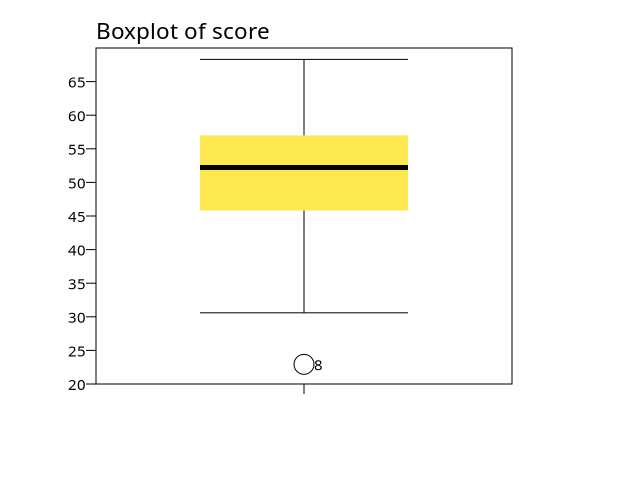
EXAMINEincludes the Shapiro-Wilk normality test in its output. A small p-value indicates the variable is not normally distributed.INPUT PROGRAM. LOOP #i = 1 TO 50. COMPUTE score = RV.NORMAL(50, 10). END CASE. END LOOP. END FILE. END INPUT PROGRAM. EXAMINE VARIABLES = score /STATISTICS = DESCRIPTIVES /PLOT = ALL.Case Processing Summary +-----+-------------------------------+ | | Cases | | +----------+---------+----------+ | | Valid | Missing | Total | | +--+-------+-+-------+--+-------+ | | N|Percent|N|Percent| N|Percent| +-----+--+-------+-+-------+--+-------+ |score|50| 100.0%|0| .0%|50| 100.0%| +-----+--+-------+-+-------+--+-------+See examine4-1.png for a chart.
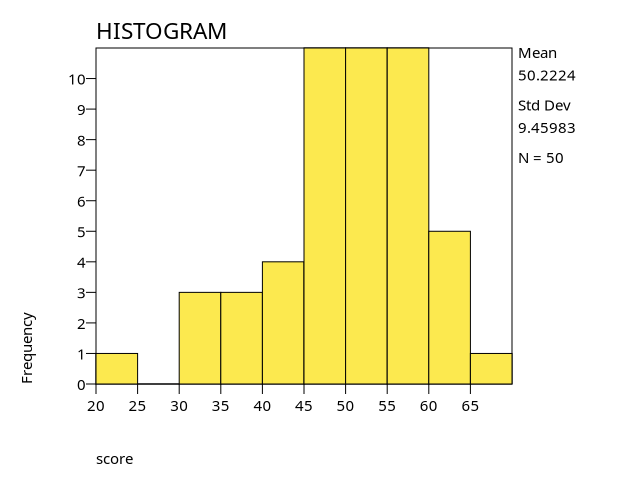
See examine4-2.png for a chart.
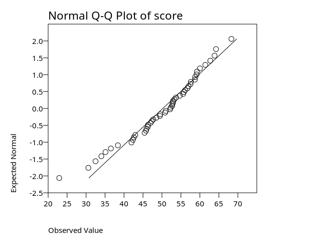
See examine4-3.png for a chart.
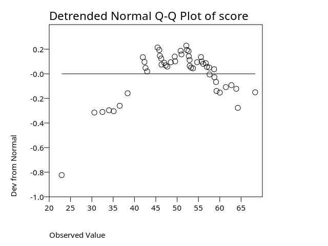
See examine4-4.png for a chart.
                               Descriptives
+--------------------------------------------------+---------+----------+
|                                                  |Statistic|Std. Error|
+--------------------------------------------------+---------+----------+
|score Mean                                        |    50.22|      1.34|
|     ---------------------------------------------+---------+----------+
|      95% Confidence Interval for Mean Lower Bound|    47.53|          |
|                                       Upper Bound|    52.91|          |
|     ---------------------------------------------+---------+----------+
|      5% Trimmed Mean                             |    50.60|          |
|     ---------------------------------------------+---------+----------+
|      Median                                      |    52.22|          |
|     ---------------------------------------------+---------+----------+
|      Variance                                    |    89.49|          |
|     ---------------------------------------------+---------+----------+
|      Std. Deviation                              |     9.46|          |
|     ---------------------------------------------+---------+----------+
|      Minimum                                     |    22.93|          |
|     ---------------------------------------------+---------+----------+
|      Maximum                                     |    68.30|          |
|     ---------------------------------------------+---------+----------+
|      Range                                       |    45.38|          |
|     ---------------------------------------------+---------+----------+
|      Interquartile Range                         |    11.41|          |
|     ---------------------------------------------+---------+----------+
|      Skewness                                    |     -.69|       .34|
|     ---------------------------------------------+---------+----------+
|      Kurtosis                                    |      .44|       .66|
+--------------------------------------------------+---------+----------+

    Tests of Normality
+-----+-----------------+
|     |   Shapiro-Wilk  |
|     +---------+--+----+
|     |Statistic|df|Sig.|
+-----+---------+--+----+
|score|      .97|50| .19|
+-----+---------+--+----+
EXAMINEprovides descriptive statistics and several diagnostic plots for the variable. The output includes the mean, standard deviation, normality test, and the associated charts. This example demonstrates typical results when using/STATISTICS = DESCRIPTIVESand/PLOT = ALLon a reasonably sized dataset.Next, PSPP’s
REGRESSIONcommand performs ordinary least squares estimation. The following section shows a simple regression example and the standard output produced by PSPP.How to Run a Linear Regression
The
REGRESSIONcommand fits an ordinary least squares model to a continuous dependent variable using one or more numeric predictors. After checking the variables withFREQUENCIESandCROSSTABS, regression shows how the outcome relates to the predictors. PSPP provides the standard coefficients and model statistics used in OLS (ordinary least squares).DATA LIST LIST / y x1 x2. BEGIN DATA 10 1 4.1 12 2 5.0 13 3 6.2 15 4 7.1 16 5 8.0 END DATA. LIST. REGRESSION /DEPENDENT = y /METHOD = ENTER x1 x2 /STATISTICS = COEFF R ANOVA /SAVE = PRED RESID.Output:
This
/SAVEoption above creates two additional variables:PRED1(predicted values) andRES1(residuals).Workflow Tip: Many statistics courses require students to examine and plot the residuals and predicted values to check model assumptions. Saving these values in PSPP's regression procedure provides exactly what those assignments need.
    Data List
╭─────┬────┬────╮
│  y  │ x1 │ x2 │
├─────┼────┼────┤
│10.00│1.00│4.10│
│12.00│2.00│5.00│
│13.00│3.00│6.20│
│15.00│4.00│7.10│
│16.00│5.00│8.00│
╰─────┴────┴────╯
                     Model Summary (y)
╭───┬────────┬─────────────────┬──────────────────────────╮
│ R │R Square│Adjusted R Square│Std. Error of the Estimate│
├───┼────────┼─────────────────┼──────────────────────────┤
│.99│     .99│              .98│                       .37│
╰───┴────────┴─────────────────┴──────────────────────────╯
                      ANOVA (y)
╭──────────┬──────────────┬──┬───────────┬─────┬────╮
│          │Sum of Squares│df│Mean Square│  F  │Sig.│
├──────────┼──────────────┼──┼───────────┼─────┼────┤
│Regression│         22.53│ 2│      11.27│84.50│.012│
│Residual  │           .27│ 2│        .13│     │    │
│Total     │         22.80│ 4│           │     │    │
╰──────────┴──────────────┴──┴───────────┴─────┴────╯
                               Coefficients (y)
╭──────────┬────────────────────────────┬─────────────────────────┬────┬────╮
│          │ Unstandardized Coefficients│Standardized Coefficients│    │    │
│          ├───────────┬────────────────┼─────────────────────────┤    │    │
│          │     B     │   Std. Error   │           Beta          │  t │Sig.│
├──────────┼───────────┼────────────────┼─────────────────────────┼────┼────┤
│(Constant)│      12.16│            6.92│                      .00│1.76│.177│
│x1        │       2.60│            2.20│                     1.72│1.18│.359│
│x2        │      -1.11│            2.22│                     -.73│-.50│.667│
╰──────────┴───────────┴────────────────┴─────────────────────────┴────┴────╯

LIST.

          Data List
╭─────┬────┬────┬────┬─────╮
│  y  │ x1 │ x2 │RES1│PRED1│
├─────┼────┼────┼────┼─────┤
│10.00│1.00│4.10│-.20│10.20│
│12.00│2.00│5.00│ .20│11.80│
│13.00│3.00│6.20│-.07│13.07│
│15.00│4.00│7.10│ .33│14.67│
│16.00│5.00│8.00│-.27│16.27│
╰─────┴────┴────┴────┴─────╯
The output includes the standard tables for an ordinary least squares model. The Model Summary shows an R of 0.99 and an R‑square of 0.99 for this small example. The Coefficients table lists each predictor along with its estimate, standard error, t-statistic, and p‑value. These values confirm that the procedure ran correctly and that PSPP produced the expected regression statistics. Interpretation of the coefficients depends on the context and the analyst’s goals; the purpose here is simply to show how PSPP fits the model and reports the results.
Scatterplot of predicted vs residuals.
Code:
** Use regression output variables (pred and resid) to check data.
GRAPH
  /SCATTERPLOT = pred1 WITH res1.
Output:
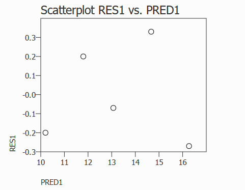
All we see is a cloud of points and there is no trend or pattern. This is what we'd like to see from residuals: a random scatter with no pattern. With only 5 points, the plot is naturally sparse, but it still shows no systematic pattern (but note it's easy to be fooled by a few points).
Note: psppire exports the entire output window, not individual plots. To save a plot for documentation or reports, use your system’s screenshot tool to capture just the graphic from the Output window.
Note: PSPP accepts the SPSS BIVAR keyword in scatterplots for compatibility, but it has no effect on the plot. PSPP always produces a simple bivariate scatterplot.
How to Compute the P-value for the F-statistic Manually
PSPP can be used to compute the p-value for the F-statistic. The CDF.F function returns the cumulative distribution function of the F distribution--that is, the probability that an F‑distributed variable is less than or equal to the specified value.
The following calculates the upper tail probability for an F value of 84.50 with 2 model and 2 error degrees of freedom, as shown in the ANOVA table from the regression output.
DO IF $CASENUM = 1.
  COMPUTE p_F = 1 - CDF.F(84.50, 2, 2).
END IF.
FORMATS p_F (F10.6).
LIST p_F /CASES=FROM 1 TO 1.

Data List
╭───────╮
│  p_F  │
├───────┤
│.011696│
╰───────╯
The computed p-value is 0.011696 which matches the pspp output within rounding error. The
DO IFblock runs theCOMPUTEexpression only for the first case, and theLISTcommand displays only that case. All remaining cases contain system-missing values forp_F.Workflow Tip: PSPP does not have standalone scalar variables, so computing a single value (such as a p‑value or critical value) is done by attaching the calculation to the first case in the active dataset. Using
DO IF $CASENUM = 1and listing only that case prints the computed value without producing output for all other cases.How to Run a Oneway Analysis of Variance (ONEWAY)
The
ONEWAYprocedure tests whether the mean of a numeric variable differs across two or more independent groups. It is the simplest form of ANOVA and is useful when you have one factor (a categorical variable) and one dependent variable. PSPP produces the standard ANOVA table along with optional descriptive statistics, homogeneity tests, and post‑hoc comparisons.ONEWAYoperates on the active dataset, so you must read data into PSPP before running the procedure. Once the data is loaded,ONEWAYprovides a quick way to compare group means and determine whether any differences are statistically significant.Using psppire for Oneway: Run a one-way ANOVA through Analyze -> Compare Means -> One-Way ANOVA.
PSPPIRE supports selecting the dependent variable and factor, requesting descriptive statistics, and choosing post‑hoc tests. Options not available in the GUI can still be added using PSPP syntax.
psppire displays the same tables as the syntax version.
DATA LIST LIST /group score hours gpa passed major age.
BEGIN DATA
1  72  3 2.8 1 1 19
1  75  4 3.0 1 1 20
1  68  2 2.5 0 1 18
2  81  5 3.4 1 2 21
2  79  4 3.2 1 2 22
2  74  3 3.0 0 2 20
3  90  6 3.8 1 3 23
3  88  5 3.6 1 3 22
3  85  5 3.5 1 3 21
END DATA.
LIST.
* Save the data.
SAVE OUTFILE='example2.sav'.

ONEWAY score BY group
  /STATISTICS DESCRIPTIVES
  /POSTHOC = TUKEY ALPHA(.05).
Reading free-form data from INLINE. Data List +-----+-----+-----+----+------+-----+-----+ |group|score|hours| gpa|passed|major| age | +-----+-----+-----+----+------+-----+-----+ | 1.00|72.00| 3.00|2.80| 1.00| 1.00|19.00| | 1.00|75.00| 4.00|3.00| 1.00| 1.00|20.00| | 1.00|68.00| 2.00|2.50| .00| 1.00|18.00| | 2.00|81.00| 5.00|3.40| 1.00| 2.00|21.00| | 2.00|79.00| 4.00|3.20| 1.00| 2.00|22.00| | 2.00|74.00| 3.00|3.00| .00| 2.00|20.00| | 3.00|90.00| 6.00|3.80| 1.00| 3.00|23.00| | 3.00|88.00| 5.00|3.60| 1.00| 3.00|22.00| | 3.00|85.00| 5.00|3.50| 1.00| 3.00|21.00| +-----+-----+-----+----+------+-----+-----+ +--------+------+ |Variable|Format| +--------+------+ |group |F8.0 | |score |F8.0 | |hours |F8.0 | |gpa |F8.0 | |passed |F8.0 | |major |F8.0 | |age |F8.0 | +--------+------+ Descriptives +-----------+-+-----+-----------+-------+---------------------+-------+-------+ | | | | | | 95% Confidence | | | | | | | | | Interval for Mean | | | | | | | | +----------+----------+ | | | | | | Std. | Std. | Lower | Upper | | | | group|N| Mean| Deviation | Error | Bound | Bound |Minimum|Maximum| +-----------+-+-----+-----------+-------+----------+----------+-------+-------+ |score 1.00 |3|71.67| 3.51| 2.03| 62.94| 80.39| 68.00| 75.00| | 2.00 |3|78.00| 3.61| 2.08| 69.04| 86.96| 74.00| 81.00| | 3.00 |3|87.67| 2.52| 1.45| 81.42| 93.92| 85.00| 90.00| | Total|9|79.11| 7.52| 2.51| 73.33| 84.89| 68.00| 90.00| +-----------+-+-----+-----------+-------+----------+----------+-------+-------+ ANOVA +--------------------+--------------+--+-----------+-----+----+ | |Sum of Squares|df|Mean Square| F |Sig.| +--------------------+--------------+--+-----------+-----+----+ |score Between Groups| 389.56| 2| 194.78|18.45|.003| | Within Groups | 63.33| 6| 10.56| | | | Total | 452.89| 8| | | | +--------------------+--------------+--+-----------+-----+----+ Multiple Comparisons (score) +--------------------------+-----------------+--------+----+------------------+ | | | | | 95% Confidence | | | | | | Interval | | | | | +---------+--------+ | (I) (J) | Mean Difference | Std. | | Lower | Upper | | Family Family | (I - J) | Error |Sig.| Bound | Bound | +--------------------------+-----------------+--------+----+---------+--------+ |Tukey 1.00 2.00 | -6.33| 2.65|.118| -14.47| 1.81| |HSD 3.00 | -16.00| 2.65|.002| -24.14| -7.86| | -------------------+-----------------+--------+----+---------+--------+ | 2.00 1.00 | 6.33| 2.65|.118| -1.81| 14.47| | 3.00 | -9.67| 2.65|.025| -17.81| -1.53| | -------------------+-----------------+--------+----+---------+--------+ | 3.00 1.00 | 16.00| 2.65|.002| 7.86| 24.14| | 2.00 | 9.67| 2.65|.025| 1.53| 17.81| +--------------------------+-----------------+--------+----+---------+--------+The data set read correctly. The ONEWAY procedure ANOVA table shows that the group means are significantly different (p=0.003). Tukey post hoc comparisons indicate that family 1 and 3 differ signifcantly as do family 2 and 3. But family 1 and 2 do not differ significantly.
How to Run a Oneway Analysis of Variance (GLM)
Another way to run a Oneway Analysis of Variance is with the
GLMprocedure.GLMstands for General Linear Model. For a single factor the model is the same as for theONEWAYcommand.GLMdoesn't have all the extra statistics and comparisons, though.DATA LIST LIST /group score hours gpa passed major age. BEGIN DATA 1 72 3 2.8 1 1 19 1 75 4 3.0 1 1 20 1 68 2 2.5 0 1 18 2 81 5 3.4 1 2 21 2 79 4 3.2 1 2 22 2 74 3 3.0 0 2 20 3 90 6 3.8 1 3 23 3 88 5 3.6 1 3 22 3 85 5 3.5 1 3 21 END DATA. LIST. * Save the data. SAVE OUTFILE='example2.sav'. GLM score BY group /DESIGN = group. EXECUTE.Reading free-form data from INLINE. +--------+------+ |Variable|Format| +--------+------+ |group |F8.0 | |score |F8.0 | |hours |F8.0 | |gpa |F8.0 | |passed |F8.0 | |major |F8.0 | |age |F8.0 | +--------+------+ Data List +-----+-----+-----+----+------+-----+-----+ |group|score|hours| gpa|passed|major| age | +-----+-----+-----+----+------+-----+-----+ | 1.00|72.00| 3.00|2.80| 1.00| 1.00|19.00| | 1.00|75.00| 4.00|3.00| 1.00| 1.00|20.00| | 1.00|68.00| 2.00|2.50| .00| 1.00|18.00| | 2.00|81.00| 5.00|3.40| 1.00| 2.00|21.00| | 2.00|79.00| 4.00|3.20| 1.00| 2.00|22.00| | 2.00|74.00| 3.00|3.00| .00| 2.00|20.00| | 3.00|90.00| 6.00|3.80| 1.00| 3.00|23.00| | 3.00|88.00| 5.00|3.60| 1.00| 3.00|22.00| | 3.00|85.00| 5.00|3.50| 1.00| 3.00|21.00| +-----+-----+-----+----+------+-----+-----+ Tests of Between-Subjects Effects +---------------+-----------------------+--+-----------+-------+----+ | |Type III Sum Of Squares|df|Mean Square| F |Sig.| +---------------+-----------------------+--+-----------+-------+----+ |Corrected Model| 389.56| 2| 194.78| 18.45|.003| |Intercept | 56327.11| 1| 56327.11|5336.25|.000| |group | 389.56| 2| 194.78| 18.45|.003| |Error | 63.33| 6| 10.56| | | |Total | 56780.00| 9| | | | |Corrected Total| 452.89| 8| | | | +---------------+-----------------------+--+-----------+-------+----+GLM gives you the Intercept while ONEWAY doesn't display it. The results are the same as from ONEWAY on the same data. F is 18.45 with 2 and 6 degrees of freedom) and p=0.003.
How to Run a RELIABILITY Analysis
The
RELIABILITYcommand computes internal consistency statistics for a set of variables. PSPP currently supports Cronbach’s alpha and split‑half reliability. This example shows a simple alpha calculation for a group of items. The PSPP GUI does not have Reliability in its menus but the code can be run in the Syntax Editor or from the command line.PSPP Code:
SET FORMAT=F8.5.
SET WIDTH=132
    /LENGTH=59
    /MXLOOPS=100
    /RESULTS=BOTH.
TITLE 'Reliability Analysis'.

GET FILE='study.sys'.

RELIABILITY /VARIABLES=FEELRUSH TO FEELSMAL.

FINISH.
Output:
Scale: ANY

Case Processing Summary
+--------+--+-------+
|Cases   | N|Percent|
+--------+--+-------+
|Valid   |93|  93.9%|
|Excluded| 6|   6.1%|
|Total   |99| 100.0%|
+--------+--+-------+

    Reliability Statistics
+----------------+----------+
|Cronbach's Alpha|N of Items|
+----------------+----------+
|          .84949|        20|
+----------------+----------+
PSPP’s reliability procedure provides a case summary and Cronbach’s alpha for the specified variables. This is sufficient for checking basic internal consistency in most datasets. A high value of Cronback's alpha means the items are correlated, but not necessarily that the scale is valid or meaningful.
T-TEST
The T-TEST procedure compares means between one or two groups or between two related measurements. PSPP supports one-sample, independent samples, and paired-samples T-tests.
Three Examples of T-test
Data:
group  score  pretest  posttest
1      42     40       48
1      55     52       58
1      47     45       50
2      60     58       62
2      65     63       68
2      70     67       72
One-sample T-test
Code:
T-TEST
  /TESTVAL = 50
  /VARIABLES = score.

T-TEST
  /GROUPS = group(1 2)
  /VARIABLES = score.

T-TEST
  /PAIRS = pretest WITH posttest.
Output:
DATA LIST LIST /group score pretest posttest.
Reading free-form data from INLINE.
╭────────┬──────╮
│Variable│Format│
├────────┼──────┤
│group   │F8.0  │
│score   │F8.0  │
│pretest │F8.0  │
│posttest│F8.0  │
╰────────┴──────╯
BEGIN DATA
 1      42     40       48
 1      55     52       58
 1      47     45       50
 2      60     58       62
 2      65     63       68
 2      70     67       72
END DATA.
LIST.
           Data List
╭─────┬─────┬───────┬────────╮
│group│score│pretest│posttest│
├─────┼─────┼───────┼────────┤
│ 1.00│42.00│  40.00│   48.00│
│ 1.00│55.00│  52.00│   58.00│
│ 1.00│47.00│  45.00│   50.00│
│ 2.00│60.00│  58.00│   62.00│
│ 2.00│65.00│  63.00│   68.00│
│ 2.00│70.00│  67.00│   72.00│
╰─────┴─────┴───────┴────────╯

T-TEST
  /TESTVAL = 50
  /VARIABLES = score.
          One-Sample Statistics
╭─────┬─┬─────┬──────────────┬─────────╮
│     │N│ Mean│Std. Deviation│S.E. Mean│
├─────┼─┼─────┼──────────────┼─────────┤
│score│6│56.50│         10.67│     4.36│
╰─────┴─┴─────┴──────────────┴─────────╯
                                      One-Sample Test
╭─────┬──────────────────────────────────────────────────────────────────────────────────╮
│     │                                  Test Value = 50                                 │
│     ├────┬──┬───────────────┬───────────────┬──────────────────────────────────────────┤
│     │    │  │               │               │ 95% Confidence Interval of the Difference│
│     │    │  │               │               ├─────────────────────┬────────────────────┤
│     │  t │df│Sig. (2-tailed)│Mean Difference│        Lower        │        Upper       │
├─────┼────┼──┼───────────────┼───────────────┼─────────────────────┼────────────────────┤
│score│1.49│ 5│           .196│           6.50│                -4.70│               17.70│
╰─────┴────┴──┴───────────────┴───────────────┴─────────────────────┴────────────────────╯
Independent Samples T-Test
T-TEST
  /GROUPS = group(1 2)
  /VARIABLES = score.

               Group Statistics
╭───────────┬─┬─────┬──────────────┬─────────╮
│      Group│N│ Mean│Std. Deviation│S.E. Mean│
├───────────┼─┼─────┼──────────────┼─────────┤
│score 1.00 │3│48.00│          6.56│     3.79│
│      2.00 │3│65.00│          5.00│     2.89│
╰───────────┴─┴─────┴──────────────┴─────────╯
                                                                                Independent Samples Test
╭─────────────────────────────────┬────────────────────────────────────────┬───────────────────────────────────────────────────────────────────────────────────────────────────────────╮
│                                 │ Levene's Test for Equality of Variances│                                        T-Test for Equality of Means                                       │
│                                 ├──────────────────┬─────────────────────┼─────┬────┬───────────────┬───────────────┬─────────────────────┬──────────────────────────────────────────┤
│                                 │                  │                     │     │    │               │               │                     │ 95% Confidence Interval of the Difference│
│                                 │                  │                     │     │    │               │               │                     ├─────────────────────┬────────────────────┤
│                                 │         F        │         Sig.        │  t  │ df │Sig. (2-tailed)│Mean Difference│Std. Error Difference│        Lower        │        Upper       │
├─────────────────────────────────┼──────────────────┼─────────────────────┼─────┼────┼───────────────┼───────────────┼─────────────────────┼─────────────────────┼────────────────────┤
│score Equal variances assumed    │               .29│                 .621│-3.57│4.00│           .023│         -17.00│                 4.76│               -30.22│               -3.78│
│      Equal variances not assumed│                  │                     │-3.57│3.74│           .026│         -17.00│                 4.76│               -30.59│               -3.41│
╰─────────────────────────────────┴──────────────────┴─────────────────────┴─────┴────┴───────────────┴───────────────┴─────────────────────┴─────────────────────┴────────────────────╯
Paired Samples T-test
T-TEST
  /PAIRS = pretest WITH posttest.

             Paired Sample Statistics
╭───────────────┬─┬─────┬──────────────┬─────────╮
│               │N│ Mean│Std. Deviation│S.E. Mean│
├───────────────┼─┼─────┼──────────────┼─────────┤
│Pair 1 pretest │6│54.17│         10.46│     4.27│
│       posttest│6│59.67│          9.58│     3.91│
╰───────────────┴─┴─────┴──────────────┴─────────╯
          Paired Samples Correlations
╭─────────────────────────┬─┬───────────┬────╮
│                         │N│Correlation│Sig.│
├─────────────────────────┼─┼───────────┼────┤
│Pair 1 pretest & posttest│6│       .994│.000│
╰─────────────────────────┴─┴───────────┴────╯
                                                      Paired Samples Test
╭─────────────────────────┬─────────────────────────────────────────────────────────────────────────┬─────┬──┬───────────────╮
│                         │                            Paired Differences                           │     │  │               │
│                         ├─────┬──────────────┬─────────┬──────────────────────────────────────────┤     │  │               │
│                         │     │              │         │ 95% Confidence Interval of the Difference│     │  │               │
│                         │     │              │         ├─────────────────────┬────────────────────┤     │  │               │
│                         │ Mean│Std. Deviation│S.E. Mean│        Lower        │        Upper       │  t  │df│Sig. (2-tailed)│
├─────────────────────────┼─────┼──────────────┼─────────┼─────────────────────┼────────────────────┼─────┼──┼───────────────┤
│Pair 1 pretest - posttest│-5.50│          1.38│      .56│                -6.95│               -4.05│-9.77│ 5│           .000│
╰─────────────────────────┴─────┴──────────────┴─────────┴─────────────────────┴────────────────────┴─────┴──┴───────────────╯
The T‑test compares means and reports whether the observed difference is larger than what would be expected by chance. PSPP reports the t‑value, degrees of freedom, and the two‑tailed significance level (p‑value). A small p‑value indicates that the difference between means is unlikely to be due to sampling variation alone. For independent‑samples tests, PSPP also reports Levene’s test for equality of variances; use the appropriate row based on that result. For paired‑samples tests, the difference is computed within subjects.
RANK
The RANK procedure assigns an order number to values in a data set based on several rules. One of the main things about ranking values is how the tied values are handled. The default method used by PSPP is the MEAN of the ranks that would be applied to the tied values if we didn't handle them another way. If the ranks assigned were 1, 2, 3, etc. without regard to tied values I'd call these the base ranks. They are not the final ranks, but an intermediate step to handling tied values.
The following examples show how each tie-handling method works. Each method is demonstrated with the same data, and each produces a new variable containing the ranks assigned under that method.
Workflow tip: PSPP does not allow multiple output variables in a single
/RANK INTOclause. To produce ranks using different tie methods, run the RANK command multiple times, each with its own/TIES=setting.In the first example below, the RANK procedure is run and the mean method is specified (it is the default if you don't specify any tie method).
DATA LIST LIST /X .

Reading free-form data from INLINE.
╭────────┬──────╮
│Variable│Format│
├────────┼──────┤
│X       │F8.0  │
╰────────┴──────╯
BEGIN DATA.
 0
 0
 0
 1
 1
 3
END DATA.

LIST.
Data List
╭────╮
│  X │
├────┤
│ .00│
│ .00│
│ .00│
│1.00│
│1.00│
│3.00│
╰────╯
RANK
  VARIABLES = x
  /RANK INTO r_mean

  /TIES = MEAN .
        Variables Created by RANK
╭─────────────────┬────────────┬────────╮
│Existing Variable│New Variable│Function│
├─────────────────┼────────────┼────────┤
│X                │r_mean      │RANK    │
╰─────────────────┴────────────┴────────╯

  LIST /r_mean.

Data List
╭──────╮
│r_mean│
├──────┤
│ 2.000│
│ 2.000│
│ 2.000│
│ 4.500│
│ 4.500│
│ 6.000│
╰──────╯
0, 0, 0, 1, 1, 3 gives us base ranks of 1, 2, 3, 4, 5, 6. With 0, 0, 0. ranked as 1, 2, 3, the mean of the ranks is taken from 1+2+3/3=2. For the 1, 1 values the mean of the base ranks of 4 and 5 becomes ranks of 4.5. The resulting ranks should be 2, 2, 2, 4.5, 4.5, and 6, which is how they came out.
The LOW method for ties chooses the lowest base rank for a set of ties and applies it to the ties in that set of values. 0, 0, 0, 1, 1, 3 with base ranks of 1, 2, 3, 4, 5, 6 gives 1, 1, 1, 4, 4, 6. The low value of 1, 2, 3 is 1, and low value of 4, 5, is 4.
  RANK
  VARIABLES = x
  /RANK INTO r_low
  /TIES = LOW.
        Variables Created by RANK
╭─────────────────┬────────────┬────────╮
│Existing Variable│New Variable│Function│
├─────────────────┼────────────┼────────┤
│X                │r_low       │RANK    │
╰─────────────────┴────────────┴────────╯

  LIST /r_low.

Data List
╭─────╮
│r_low│
├─────┤
│1.000│
│1.000│
│1.000│
│4.000│
│4.000│
│6.000│
╰─────╯
The HIGH method for ties chooses the highest base rank for a set of ties. 0, 0, 0, 1, 1, 3 with base ranks of 1, 2, 3, 4, 5, 6 would result in 3, 3, 3, 5, 5, 6.
  RANK
  VARIABLES = x
  /RANK INTO r_high
  /TIES = HIGH.
        Variables Created by RANK
╭─────────────────┬────────────┬────────╮
│Existing Variable│New Variable│Function│
├─────────────────┼────────────┼────────┤
│X                │r_high      │RANK    │
╰─────────────────┴────────────┴────────╯

  LIST /r_high.

Data List
╭──────╮
│r_high│
├──────┤
│ 3.000│
│ 3.000│
│ 3.000│
│ 5.000│
│ 5.000│
│ 6.000│
╰──────╯
The CONDENSE method assigns consecutive ranks to distinct values ignoring base ranks entirely. All cases with the same value get the same rank. This results in a rank variable with no gaps in ranks and no fractional ranks. 0, 0, 0, 1, 1, 3 ranks to 1, 1, 1, 2, 2, 3.
  RANK
  VARIABLES = x
  /RANK INTO r_cond
  /TIES = CONDENSE.
        Variables Created by RANK
╭─────────────────┬────────────┬────────╮
│Existing Variable│New Variable│Function│
├─────────────────┼────────────┼────────┤
│X                │r_cond      │RANK    │
╰─────────────────┴────────────┴────────╯

  LIST r_cond.

Data List
╭──────╮
│r_cond│
├──────┤
│ 1.000│
│ 1.000│
│ 1.000│
│ 2.000│
│ 2.000│
│ 3.000│
╰──────╯
The
RANKprocedure is useful whenever the order of values matters more than their actual numeric size. Ranking is the foundation of many nonparametric tests (such as Mann–Whitney, Wilcoxon, Kruskal–Wallis, and Spearman correlations), and it is also helpful when the data are skewed, contain outliers, or are measured on an ordinal scale. By converting raw values into ranks, PSPP lets you analyze the relative positions of cases without assuming anything about the underlying distribution of the data.CORRELATIONS
PSPP currently supports only Pearson product–moment correlations. This
CORRELATIONSprocedure is intended for exploratory analysis — inspecting linear relationships between variables and checking whether variables tend to move together.PSPP does not provide:
- Spearman or Kendall correlations
- Partial correlations
- Options to save the correlation matrix to a file
- Export of the matrix for use in other procedures
The output is for inspection only.
Two options for
CORRELATIONSare how missing data are to be handled. They areLISTWISEandPAIRWISE. With LISTWISE, a case is included only if it has valid data for all variables. PAIRWISE tells the procedure to use all cases valid for each pair of variables. PAIRWISE is the default setting.Code:
DATA LIST LIST /group score hours gpa passed major age.
BEGIN DATA
1  72  3 2.8 1 1 19
1  75  4 3.0 1 1 20
1  68  2 2.5 0 1 18
2  81  5 3.4 1 2 21
2  79  4 3.2 1 2 22
2  74  3 3.0 0 2 20
3  90  6 3.8 1 3 23
3  88  5 3.6 1 3 22
3  85  5 3.5 1 3 21
END DATA.
LIST.

CORRELATIONS
  /VARIABLES = score hours
  /MISSING = LISTWISE.
EXECUTE.
Output:
 DATA LIST LIST /group score hours gpa passed major age.
Reading free-form data from INLINE.
╭────────┬──────╮
│Variable│Format│
├────────┼──────┤
│group   │F8.0  │
│score   │F8.0  │
│hours   │F8.0  │
│gpa     │F8.0  │
│passed  │F8.0  │
│major   │F8.0  │
│age     │F8.0  │
╰────────┴──────╯
BEGIN DATA
1  72  3 2.8 1 1 19
1  75  4 3.0 1 1 20
1  68  2 2.5 0 1 18
2  81  5 3.4 1 2 21
2  79  4 3.2 1 2 22
2  74  3 3.0 0 2 20
3  90  6 3.8 1 3 23
3  88  5 3.6 1 3 22
3  85  5 3.5 1 3 21
END DATA.
                 Data List
╭─────┬─────┬─────┬────┬──────┬─────┬─────╮
│group│score│hours│ gpa│passed│major│ age │
├─────┼─────┼─────┼────┼──────┼─────┼─────┤
│ 1.00│72.00│ 3.00│2.80│  1.00│ 1.00│19.00│
│ 1.00│75.00│ 4.00│3.00│  1.00│ 1.00│20.00│
│ 1.00│68.00│ 2.00│2.50│   .00│ 1.00│18.00│
│ 2.00│81.00│ 5.00│3.40│  1.00│ 2.00│21.00│
│ 2.00│79.00│ 4.00│3.20│  1.00│ 2.00│22.00│
│ 2.00│74.00│ 3.00│3.00│   .00│ 2.00│20.00│
│ 3.00│90.00│ 6.00│3.80│  1.00│ 3.00│23.00│
│ 3.00│88.00│ 5.00│3.60│  1.00│ 3.00│22.00│
│ 3.00│85.00│ 5.00│3.50│  1.00│ 3.00│21.00│
╰─────┴─────┴─────┴────┴──────┴─────┴─────╯

CORRELATIONS
  /VARIABLES = score hours
  /MISSING = LISTWISE.
              Correlations
╭─────────────────────────┬─────┬─────╮
│                         │score│hours│
├─────────────────────────┼─────┼─────┤
│score Pearson Correlation│1.000│ .954│
│      Sig. (2-tailed)    │     │ .000│
├─────────────────────────┼─────┼─────┤
│hours Pearson Correlation│ .954│1.000│
│      Sig. (2-tailed)    │ .000│     │
╰─────────────────────────┴─────┴─────╯
Interpretation:
Score and hours are strongly positively correlated (r = .954). This means that cases with higher hours tend to have higher scores, and cases with lower hours tend to have lower scores. The relationship is strong and consistent.
Important: Correlation does not necessarily imply causation
A classic example is that suicide rates and ice cream sales are strongly correlated, but neither one causes the other. Both tend to rise during warmer months, so the relationship is driven by a third factor (seasonality), not a direct causal link.
Correlation describes how variables move together — not why.
NPAR TESTS
Nonparametric tests generally work on ranks rather than raw values, although some nonparametric procedures operate on counts, medians, or signs (such as the median or signs tests) instead. They make few assumptions about the data distributions.
PSPP includes exact methods for nonparametric tests when exact computation is feasible. Exact tests are useful for small samples where asymptotic approximations may not be reliable.
The following examples show several commonly used nonparametric tests available in PSPP, including the Mann–Whitney, Wilcoxon signed‑rank, Kruskal–Wallis, and Median tests.
MANN-WHITNEY (M-W) Test (Two Independent Groups)
Code:
DATA LIST LIST /score group.
BEGIN DATA
12 1
15 1
18 1
20 1
14 2
17 2
19 2
22 2
END DATA.

NPAR TESTS
  /MANN-WHITNEY = score BY group(1, 2).
Output:
DATA LIST LIST /score group.
Reading free-form data from INLINE.
╭────────┬──────╮
│Variable│Format│
├────────┼──────┤
│score   │F8.0  │
│group   │F8.0  │
╰────────┴──────╯
BEGIN DATA
12 1
15 1
18 1
20 1
14 2
17 2
19 2
22 2
END DATA.

NPAR TESTS
  /MANN-WHITNEY = score BY group(1, 2).
                 Ranks
╭───────────┬─┬─────────┬────────────╮
│           │N│Mean Rank│Sum of Ranks│
├───────────┼─┼─────────┼────────────┤
│score 1.00 │4│     4.00│       16.00│
│      2.00 │4│     5.00│       20.00│
│      Total│8│         │            │
╰───────────┴─┴─────────┴────────────╯
                       Test Statistics
╭─────┬──────────────┬──────────┬────┬──────────────────────╮
│     │Mann-Whitney U│Wilcoxon W│  Z │Asymp. Sig. (2-tailed)│
├─────┼──────────────┼──────────┼────┼──────────────────────┤
│score│          6.00│     16.00│-.58│                  .564│
╰─────┴──────────────┴──────────┴────┴──────────────────────╯
PSPP will report:
The U statistic, the Z value, the asymptotic significance and, when requested using the
/EXACTsubcommand, the exact significance.A small p‑value indicates that the two groups differ in their distributions.
WILCOXON SIGNED-RANK (Matched Pairs)
The Wilcoxon signed‑rank test compares two related measurements from the same subjects. It is a nonparametric alternative to the paired‑samples t‑test.
Code:
DATA LIST LIST /before after.
BEGIN DATA
12 15
18 20
14 17
19 21
16 18
END DATA.

NPAR TESTS
  /WILCOXON = before WITH after (PAIRED).
Output:
DATA LIST LIST /before after.
Reading free-form data from INLINE.
╭────────┬──────╮
│Variable│Format│
├────────┼──────┤
│before  │F8.0  │
│after   │F8.0  │
╰────────┴──────╯
BEGIN DATA
12 15
18 20
14 17
19 21
16 18
END DATA.

NPAR TESTS
  /WILCOXON = before WITH after (PAIRED).
                          Ranks
╭─────────────────────────────┬─┬─────────┬────────────╮
│                             │N│Mean Rank│Sum of Ranks│
├─────────────────────────────┼─┼─────────┼────────────┤
│before - after Negative Ranks│5│     3.00│       15.00│
│               Positive Ranks│0│      NaN│         .00│
│               Ties          │0│         │            │
│               Total         │5│         │            │
╰─────────────────────────────┴─┴─────────┴────────────╯
            Test Statistics
╭──────────────────────┬──────────────╮
│                      │before - after│
├──────────────────────┼──────────────┤
│Z                     │         -2.07│
│Asymp. Sig. (2-tailed)│          .038│
╰──────────────────────┴──────────────╯
PSPP reports:
- the Z statistic
- the number of positive ranks, negative ranks, and ties
- the sum of ranks and mean ranks for each direction
PSPP reports the Z value, along with the mean ranks and sum of ranks for positive and negative differences. In this example all differences are negative, so PSPP will show zero positive ranks and a nonzero sum of negative ranks. Exact significance values are available when requested using the /EXACT subcommand.
A small p‑value indicates that the paired measurements differ systematically.
KRUSKAL-WALLIS
The Kruskal–Wallis test compares three or more independent groups using ranked data. It is a nonparametric alternative to one‑way ANOVA.
DATA LIST LIST /score group.
BEGIN DATA
12 1
15 1
18 1
14 2
17 2
19 2
20 3
22 3
24 3
END DATA.
Output:
NPAR TESTS
  /KRUSKAL-WALLIS = score BY group(1, 3).

DATA LIST LIST /score group.
Reading free-form data from INLINE.
╭────────┬──────╮
│Variable│Format│
├────────┼──────┤
│score   │F8.0  │
│group   │F8.0  │
╰────────┴──────╯
BEGIN DATA
12 1
15 1
18 1
14 2
17 2
19 2
20 3
22 3
24 3
END DATA.

NPAR TESTS
  /KRUSKAL-WALLIS = score BY group(1, 3).
            Ranks
╭──────────────┬─┬─────────╮
│              │N│Mean Rank│
├──────────────┼─┼─────────┤
│score     1.00│3│     3.00│
│          2.00│3│     4.00│
│          3.00│3│     8.00│
│      Total   │9│         │
╰──────────────┴─┴─────────╯
  Test Statistics
╭───────────┬─────╮
│           │score│
├───────────┼─────┤
│Chi-Square │ 5.60│
│df         │    2│
│Asymp. Sig.│ .061│
╰───────────┴─────╯
PSPP reports the Chi‑square statistic, the mean ranks for each group, and the asymptotic significance. Exact significance values are available only when requested using the /EXACT subcommand.
A small p‑value indicates that at least one group differs from the others in its distribution.
MEDIAN TEST
The Median test compares two independent groups by splitting the combined data at the overall median and testing whether the groups differ in how many observations fall above or below that median. It is a simple nonparametric alternative to the independent‑samples t‑test.
Code:
DATA LIST LIST /score group.
BEGIN DATA
12 1
15 1
18 1
20 1
14 2
17 2
16 2
16 2
END DATA.
NPAR TESTS
  /MEDIAN = score BY group(1, 2).
Output:
DATA LIST LIST /score group.
Reading free-form data from INLINE.
╭────────┬──────╮
│Variable│Format│
├────────┼──────┤
│score   │F8.0  │
│group   │F8.0  │
╰────────┴──────╯
BEGIN DATA
12 1
15 1
18 1
20 1
14 2
17 2
16 2
16 2
END DATA.
NPAR TESTS
  /MEDIAN = score BY group(1, 2).
        Frequencies
╭──────────────┬─────────╮
│              │  group  │
│              ├────┬────┤
│              │1.00│2.00│
├──────────────┼────┼────┤
│score > Median│   2│   1│
│      ≤ Median│   2│   3│
╰──────────────┴────┴────╯
              Test Statistics
╭─────┬─┬──────┬──────────┬──┬───────────╮
│     │N│Median│Chi-Square│df│Asymp. Sig.│
├─────┼─┼──────┼──────────┼──┼───────────┤
│score│8│ 16.00│       .53│ 1│       .465│
╰─────┴─┴──────┴──────────┴──┴───────────╯
PSPP reports:
- the overall median
- the counts above and below the median for each group
- the Chi‑square statistic
- the asymptotic significance
Exact significance values are available only when requested using the /EXACT subcommand.
A small p‑value indicates that the groups differ in how their values are distributed relative to the median.
See the main pspp page on this site for data handling tips and more PSPP commands.